Joshua's Blog

TITLE: Realtime Multi-Person 2D Pose Estimation using Part Affinity Fields

AUTHOR: Zhe Cao, Tomas Simon, Shih-En Wei, Yaser Sheikh

ASSOCIATION: CMU

FROM: arXiv:1611.08050

CONTRIBUTIONS

1. a method for multi-person pose estimation is proposed that approaches the problem in a bottom-up manner to maintain realtime performance and robustness to early commitment, but utilizes global contextual information in the detection of parts and their association.
2. Part Affinity Fields (PAFs), a set of 2D vector fields, is presented, each of which encode the location and orientation of a particular limb at each position in the image domain.

METHOD

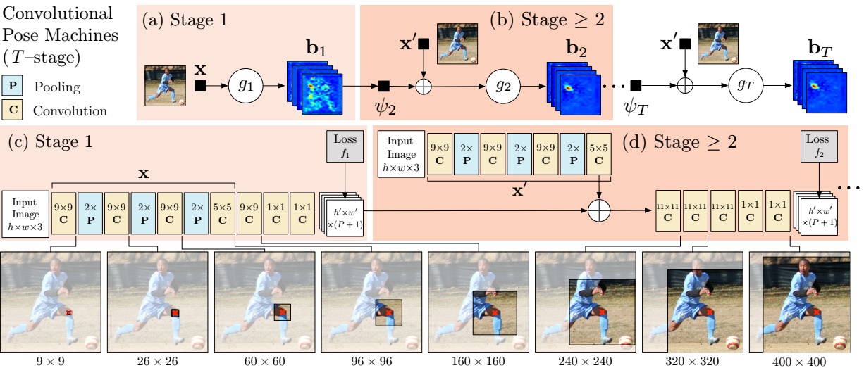
This work is the successor of Convolutional Pose Machines. The network structure, which predict the part emergence heatmap and part aafinity field jointly, is illustrated in the following figure. We can compare it with previous work.

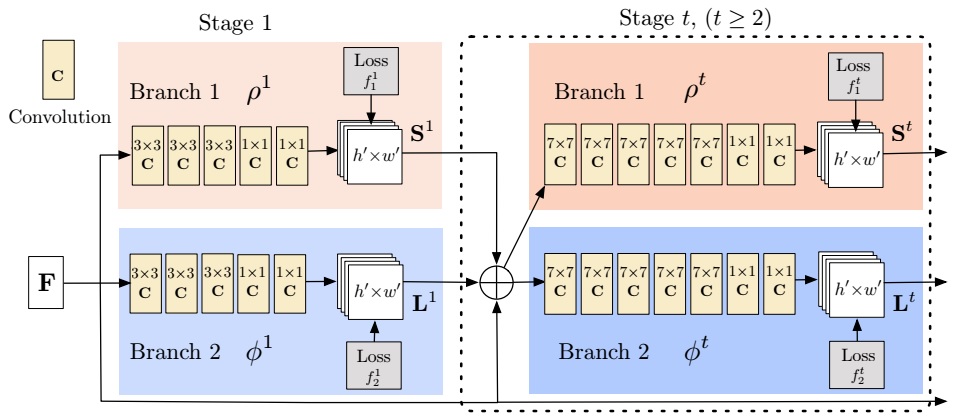
Similar with previous work, the network works as sequence learning scheme. One of the branch predicts confidence maps for part detection, while the other one predicts part affinity fields for part association.

Confidence Maps for Part Detection

At each location $ \mathbf{P} $, the value of the confidence $ S_{j}^{\ast}(\mathbf{P}) $ for a part type $ j $ is defined as

$$ S_{j}^{\ast}(\mathbf{P}) = \max \limits_{k} S_{j,k}^{\ast}(\mathbf{P}) $$

It means that for every type of part, a heatmap is predicted with multiple highlight areas, indicating the emergence of a part instance.

Part Affinity Fields for Part Association

If we consider a single limb, let $$ \mathbf{x}{j_1,k} $$ and $$ \mathbf{x}{j_{2},k} $$ be the position of body parts $$ j_{1} $$ and $$ j_{2} $$ from the limb class $$ c $$ for a person $$ k $$ on the image. $$ l_{c,k} = \Vert \mathbf{x}{j{2},k} - \mathbf{x}{j{1},k} \Vert_{2} $$ is the length of the limb, and $$ \mathbf{v} = l^{−1}{c,k}(\mathbf{x}{j_{2},k} - \mathbf{x}{j{1},k}) $$ is the unit vector in the direction of the limb. The ideal part affinity vector field, $$ L^{∗}_{c,k} $$, at an image point $$ \mathbf{P} $$ as

$$ \mathbf{L}^{\ast}_{c,k}(\mathbf{P}) = \begin{cases}
\mathbf{v}& \text{if } \mathbf{P} \text{ on limb } c,k \
\mathbf{0}& \text{otherwise}
\end{cases} $$

Similar to confidence maps for part detection, part affinity fields are also predicted for all persons

$$ \mathbf{L}^{\ast}{c}(\mathbf{P}) = \frac{1}{n{p}} \sum_{k} \mathbf{L}^{\ast}_{c,k}(\mathbf{P}) $$

where $$n_{p}$$ is the number of non-zero vectos at point $$\mathbf{P}$$. The confidence score of each limb candidate is measured by

$$ E = \int_{u=0}^{u=1} \mathbf{L}{c}(\mathbf{P}(u)) \cdot \frac{\mathbf{d}{j_{2}}-\mathbf{d}{j{1}}}{\Vert \mathbf{d}{j{2}}-\mathbf{d}{j{1}} \Vert_{2}}du $$

where $$\mathbf{d}{j{1}}$$ and $$\mathbf{d}{j{2}}$$ are two detected body parts.

Multi-Person Parsing using PAFs

The last problem is to select different limbs linked in PAFs to combine as one person’s skeleton. This is a classical generalized maximum clique problem. I think in additional to the method mentioned in this paper, many other optimiaztion algorithms can be tried. These algorithms are well discussed in multi-object tracking problem.

TITLE: Convolutional Pose Machines

AUTHOR: Shih-En Wei, Varun Ramakrishna, Takeo Kanade, Yaser Sheikh

ASSOCIATION: CMU

FROM: arXiv:1602.00134

CONTRIBUTIONS

1. learning implicit spatial models via a sequential composition of convolutional architectures
2. a systematic approach to designing and training such an architecture to learn both image features and image-dependent spatial models for structured prediction tasks, without the need for any graphical model style inference.

METHOD

The following figure shows the comparison of traditional Pose Machine and Convolutional Pose Machine

Pose Machines

A pose machine consists of a sequence of multi-class predictors, $g_{t}(\cdot)$, that are trained to predict the location of each part in each level of the hierarchy. In each $stage$ $t \in {1…T}$, the classifiers $g_{t}$ predict beliefs for assigning a location to each part $Y_{p}=z, \forall z \in \mathbb{Z}$, where $\mathbb{Z}$ is the set of all locations in an image.

As illustrated in the figure (a) and (b), the image is first sent to $Stage$ $1$ and a belief map is predicted. Then the belief map and image features $x’$ are combined to sent to the following stage. As the procedure repeats, final result is predicted from the last $Stage$ $T$.

Convolutional Pose Machines

Convolutional Neural Network is naturally a sequence of stages if multiple losses and predictors are inserted at the intermediate layers. The (c) and (d) in the figure illustrated a convolutional pose machine. The sub-network in (c) plays the role of first stage. The shared network at the top-left corner in (d) is used to extract image features $x’$, which will be combined with the output of every $Stage$ $t-1$ and sent to $Stage$ $t$. In addition, the stacked convolutional layers’ perceptual field increases as deepening, which means that more contextual infomation is taken into consideration helping refine the output.

When training, every stage has its own loss function to predict parts. These losses work similar with the auxiliary classifiers in GoogleNet, which helps alleviate the problem caused by the vanishing of gradient. The network can be trained end-to-end. Compared with traditional pose machine, CMP is much easier to train. The visualization of the network can be found here

虽说我不是什么信徒，但是这圣诞节的气氛还是挺感染人的，今天加了一上午班总觉的怪凄惨的，再加上想解决的问题最终没有搞定，就更悲凉了。下午应景又看了《真爱至上》，也算抚慰一下受伤的心灵。这电影看了得有五六年了，每年都会翻出了再看看，虽然故事基本都背下来了，但是每次看依旧会有满满的幸福感。

这电影虽然是以圣诞节为主题，不过其中的感情应该是为各个族群所接受的普世价值吧，追求爱与被爱。除了这个，今年再看这部电影突然怀念起读硕士的日子，因为电影的开篇与结尾都是机场的场景，而我在硕士阶段做智能监控所用的数据就是机场的监控录像，其中需要检测的一种事件就是“拥抱”，当时看了很多这样的样本，当时会联想到《真爱至上》这部电影，还觉得做课题有点苦，但看这样的样本却还有点幸福。今年通过看电影开始怀念做实验了，大概是因为觉得还是年轻好。

TITLE: Beyond Skip Connections: Top-Down Modulation for Object Detection

AUTHOR: Abhinav Shrivastava, Rahul Sukthankar, Jitendra Malik, Abhinav Gupta

ASSOCIATION: CMU, UC Berkeley, Google Research

FROM: arXiv:1612.06851

CONTRIBUTIONS

In this paper top-down modulations is proposed as a way to incorporate fine details into the detection framework. The standard bottom-up, feedforward ConvNet is supplemented with a top-down modulation (TDM) network, connected using lateral connections. These connections are responsible for the modulation of lower layer filters, and the top-down network handles the selection and integration of features.

METHOD

The idea of this work is very similar with the work of Feature Pyramid Networks for Object Detection. An example of Top-Down Modulation (TDM) Network is illustrated as the following figure

TDM is integrated with the bottom-up network with lateral connections. $C_{i}$ are bottom-up, feedforward feature blocks, $L_{i}$ are the lateral modules which transform low level features for the top-down contextual pathway. Finally, $T_{j,i}$, which represent flow of top-down information from index $j$ to $i$.

In this paper, the $T$ blocks are implemented using single convolutional layer (with non-linear activation) optionally with upsampling operation. The features from $C$ (processed by $L$) and $T$ are concated then sent to a convolutional layer for combination, as the following figure shows

At training stage, one new pair of lateral and top-down modules is added at a time and trained repeatedly from a pre-trained model.

前一阵看了《血战钢锯岭》，好像很久很久没有看过这么经典风格的战争片了，看一看还挺过瘾的，不过仔细想想这片好像不能只算是战争片，更多的可能算宗教篇。

耶稣说：“我就是道路、真理、生命”，整部电影的推进也差不多就是这三部分。道路篇基本就是戴斯蒙德·道斯参军前，讲述了戴斯蒙德如何因为误伤兄弟而受到神启、因为父亲差点枪杀了母亲而坚决不碰武器，又进一步进入教会成为虔诚的教徒。真理篇发生在军营，耶稣告诉我们不可杀生，但敌人该不该杀，真理何在？当戴斯蒙德经受了试炼，神迹降临，他救下了几十个战友。电影中由三个片段给我印象深刻，第一个是戴斯蒙德在清洗身上的血迹时，那是一个受洗的仪式；第二个是戴斯蒙德从山崖上下来时，战友们伸出手抚摸他，这应该是封圣，大家在迎接一个圣人；第三个是周六工作还是会被小小的惩罚一下。

TITLE: Feature Pyramid Networks for Object Detection

AUTHOR: Tsung-Yi Lin, Piotr Dollár, Ross Girshick, Kaiming He, Bharath Hariharan, Serge Belongie

ASSOCIATION: Facebook AI Research, Cornell University and Cornell Tech

FROM: arXiv:1612.03144

CONTRIBUTIONS

A new topdown architecture with lateral connections is developed for building high-level semantic feature maps at all scales is proposed. This architecture, called a Feature Pyramid Network (FPN), shows significant improvement as a generic feature extractor in several applications.

METHOD

The idea of this work is simple and is illustrated in the following figure

Similar with SSD, predictions are made in different scales. But connects exist between different scales. Though the author calls the connections as lateral connections, it is actually skip connections among different layers, just like what ResNet does.

昨天搞mxnet和caffe的混合编译，结果一直弄到今天早晨快五点，昏昏沉沉睡到了今天中午十一二点。起来后想想吃啥，发现前一阵买的辛拉面一直堆在角落里，心想不如自制一顿芝士年糕火锅吧，遂去超市买来一大堆材料，有泡菜、韩式辣椒酱、西葫芦、年糕、金针菇、午餐肉……胡乱切了切，几本就乱炖了，卖相不是太好，幸亏泡菜味道正宗，吃起来相当不错。

TITLE: Wider or Deeper: Revisiting the ResNet Model for Visual Recognition

AUTHOR: Zifeng Wu, Chunhua Shen, Anton van den Hengel

ASSOCIATION: The University of Adelaide

FROM: arXiv:1611.10080

CONTRIBUTIONS

1. A further developed intuitive view of ResNets is introduced, which helps to understand their behaviours and find possible directions to further improvements.
2. A group of relatively shallow convolutional networks is proposed based on our new understanding. Some of them achieve the state-of-the-art results on the ImageNet classification dataset.
3. The impact of using different networks is evaluated on the performance of semantic image segmentation, and these networks, as pre-trained features, can boost existing algorithms a lot.

SUMMARY

For the residual $unit \ i$, let $y_{i-1}$ be the input, and let $f_{i}(\cdot)$ be its trainable non-linear mappings, also named $Blok \ i$. The output of $unit \ i$ is recursively defined as

$$ y_{i} = f_{i}(y_{i-1}, \omega_{i})+y_{i-1} $$

where $\omega_{i}$ denotes the trainalbe parameters, and $f_{i}(\cdot)$ is often two or three stacked convolution stages in a ResNet building block. Then top left network can be formulated as

$$ y_{2} = y_{1}+f_{2}(y_{1},\omega_{2}) $$

$$ = y_{0}+f_{1}(y_{0},\omega_{1})+f_{2}(y_{0}+f_{1}(y_{0}, \omega_{1}, \omega_{2}) $$

Thus, in SGD iteration, the backward gradients are:

$$ \Delta \omega_{2}=\frac{df_{s}}{d\omega_{2}}\cdot \Delta y_{2} $$

$$ \Delta y_{1}= \Delta y_{2} + f_{2}^{‘} \cdot \Delta y_{2} $$

$$ \Delta \omega_{1} = \frac{df_{1}}{d \omega_{1}} \cdot \Delta y_{2}+ \frac{df_{1}}{d \omega_{1}} \cdot f_{2}^{‘} \cdot \Delta y_{2} $$

Ideally, when effective depth $l\geq2$, both terms of $\Delta \omega_{1}$ are non-zeros as the bottom-left case illustrated. However, when effective depth $l=1$, the second term goes to zeros, which is illustrated by the bottom-right case. If this case happens, we say that the ResNet is over-deepened, and that it cannot be trained in a fully end-to-end manner, even with those shortcut connections.

To summarize, shortcut connections enable us to train wider and deeper networks. As they growing to some point, we will face the dilemma between width and depth. From that point, going deep, we will actually get a wider network, with extra features which are not completely end-to-end trained; going wider, we will literally get a wider network, without changing its end-to-end characteristic.

The author designed three kinds of network structure as illustrated in the following figure

and the classification performance on ImageNet validation set is shown as below