TITLE: Weakly Supervised Cascaded Convolutional Networks
AUTHOR: Ali Diba, Vivek Sharma, Ali Pazandeh, Hamed Pirsiavash, Luc Van Gool
ASSOCIATION: KU Leuven, Sharif Tech., UMBC, ETH Zürich
FROM: arXiv:1611.08258
CONTRIBUTIONS
A new architecture of cascaded networks is proposed to learn a convolutional neural network handling the task without
expensive human annotations.
METHOD
This work trains a CNN to detect objects using image level annotaion, which tells what are in one image. At training stage, the input of the network are 1) original image, 2) image level labels and 3) object proposals. At inference stage, the image level labels are excluded. The object proposals can be generated by any method, such as Selective Search and EdgeBox. Two differenct cascaded network structures are proposed.
Two-stage Cascade
The two-stage cascade network structure is illustrated in the following figure.
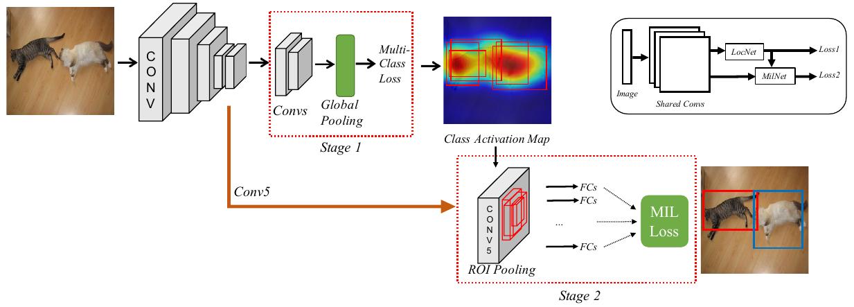
The first stage is a location network, which is a fully-convolutional CNN with a global average pooling or global maximum pooling. In order to learn multiple classes for single image, an independent loss function for each class is used. The class activation maps are used to select candidate boxes.
The second stage is multiple instance learning network. Given a bag for instances
$$ x_{c}={x_{j}|j=1,…,n} $$
and a label set
$$ y_{c}={y_{i}|y_{i} \in {0,1}, i=1,..,C } $$
where each $$ x $$ is one of the condidate boxes, $$ n $$ is the number of candidate box, $$C$$ is the number of categories and $$ \sum_{i=1}^{C}y_{i} $$, the probabilities and loss can be defined as
$$ Score(I,f_{i})=max(f_{i1},…,f_{in}) $$
$$ P(I, f_{i}) = \frac{exp(Score(I,f_{i}))}{\sum_{k=1}^{C}exp(Score(I,f_{k}))} $$
$$ L_{MIL}(P,y) = - \sum_{i=1}^{C}y_{i}log(P(I, f_i)) $$
Im my understanding, only the boxes with the most confidence in each category will be punished if they are wrong. Besides, the equations in the paper have some mistakes.
Three-stage Cascade
The three-stage cascade network structure adds a weak segmentation network between the two stages in the two-stage cascade network. It is illustrated in the following figure.
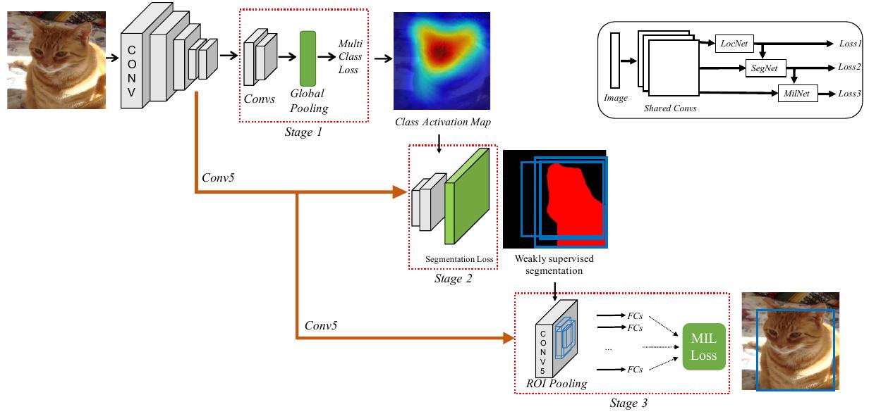
The weak segmentation network uses the results of the first stage as supervision signal. $$s_{ic}$$ is defined as the CNN score for pixel $i$ and class $$c$$ in image $I$. The score is normalized using softmax
$$ S_{ic}= exp(s_{ic})/\sum_{k=1}^{C}exp(s_{ik})$$
Considering $$y$$ as the label set for image $I$ , the loss function for the weakly supervised segmentation network is given by
$$ L_{seg}(S,G,y)=-\sum_{i=1}^{C}y_{i}log(S_{t_{c}c}) - \sum_{i \in I_{s}} \alpha_{i}log(S_{t_{c}G_{i}}) $$
$$ By \ \ \ \ \ t_{c} = \mathop{argmax}{i \in I} S{ic} $$
where $$G_{i}$$ is the supervision map for the segmentation from the first stage.
SOME IDEAS
This work requires little annotation. The only annotation is the image level label. However, this kind of training still needs complete annotation. For example, we want to detect 20 categories, then we need a 20-d vector to annotate the image. What if we only know 10/20 categories’ status in one image?