Joshua's Blog

It’s spring. Let’s go out embracing the nature!

TITLE: Deep Image Matting

AUTHOR: Ning Xu, Brian Price, Scott Cohen, Thomas Huang

ASSOCIATION: Beckman Institute for Advanced Science and Technology, University of Illinois at Urbana-Champaign, Adobe Research

FROM: arXiv:1703.03872

CONTRIBUTIONS

1. A novel deep learning based algorithm is proposed that can predict alpha matte of an image based on both low-level features and high-level context.

METHOD

The proposed deep model has two parts.

1. The first part is a CNN based encoder-decoder network, which is similar with typical FCN networks that are used for semantic segmentation. This part takes the RGB image and its corresponding trimap as input. Its output is the alpha matte of the image.
2. The second part is a small convolutional network that is used to refine the output of the first part. The input of this part is the original image and the predicted alpha matte from the first part.

The method is illustrated in the following figure.

Matting encoder-decoder stage

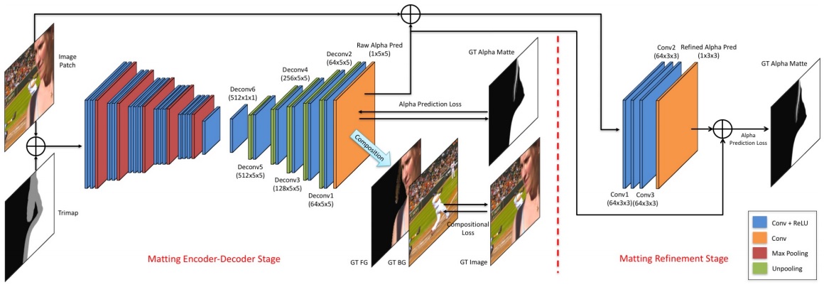
The first network leverages two losses. One is alpha-prediction loss and the other one is compositional loss.

Alpha-prediction loss is the absolute difference between the ground truth alpha values and the predicted alpha values at each pixel, which defines as

$$\mathcal{L}{\alpha}^{i} = \sqrt{(\alpha{p}^{i} - \alpha_{g}^{i})^{2}+\epsilon^2}, \alpha_{p}^{i}, \alpha_{g} \in [0,1]$$

where $\alpha_{p}^{i}$ is the output of the prediction layer at pixel $i$ and $\alpha_{g}^{i}$ is the ground truth alpha value at pixel $i$. $\epsilon$ is a small value which is equal to $10^{-1}$ and is used to ensure differentiable property.

Compositional loss the absolute difference between the ground truth RGB colors and the predicted RGB colors composited by the ground truth foreground, the ground truth background and the predicted alpha mattes. The loss is defined as

$$\mathcal{L}{c}^{i} = \sqrt{(c{p}^{i} - c_{g}^{i})^{2}+\epsilon^2}$$

where $c$ denotes the RGB channel, $p$ denotes the image composited by the predicted alpha, and $g$ denotes the image composited by the ground truth alpha.

Since only the alpha values inside the unknown regions of trimaps need to be inferred, therefore weights are set on the two types of losses according to the pixel locations, which can help the network pay more attention on the important areas. Specifically, $w_{i} = 1$ if pixel $i$ is inside the unknown region of the trimap while $w_{i} = 0$ otherwise.

Matting refinement stage

The input to the second stage of our network is the concatenation of an image patch and its alpha prediction from the first stage, resulting in a 4-channel input. This part is trained after the first part is converged. After the refinement part is also converged, finally fine-tune the the whole network together. Only the alpha prediction loss is used.

SOME IDEAS

1. The trimap is a very strong prior. The question is how to get it.

TITLE: A Pursuit of Temporal Accuracy in General Activity Detection

AUTHOR: Yuanjun Xiong, Yue Zhao, Limin Wang, Dahua Lin, Xiaoou Tang

ASSOCIATION: The Chinese University of Hong Kong, ETH

FROM: arXiv:1703.02716

CONTRIBUTIONS

1. A novel proposal scheme is proposed that can efficiently generate candidates with accurate temporal boundaries.
2. A cascaded classification pipeline is introduced that explicitly distinguishes between relevance and completeness of a candidate instance.

METHOD

The proposed action detection framework starts with evaluating the actionness of the snippets of the video. A set of temporal action proposals (in orange color) are generated with temporal actionness grouping (TAG). The proposals are evaluated against the cascaded classifiers to verify their relevance and completeness. Only proposals being complete instances are produced by the framework. Non-complete proposals and background proposals are rejected by a cascaded classification pipeline. The framework is illustrated in the following figure.

Temporal Region proposals

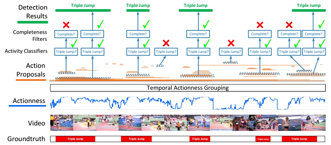
The temporal region proposals are generated with a bottom-up procedure, which consists of three steps: extract snippets, evaluate snippet-wise actionness, and finally group them into region proposals.

1. To evaluate the actionness, a binary classifier is learnt based on the Temporal Segment Network proposed in Temporal segment networks: Towards good practices for deep action recognition.
2. To generate temporal region proposals, the basic idea is to group consecutive snippets with high actionness scores. The scheme first obtains a number of action fragments by thresholding – a fragment here is a consecutive sub-sequence of snippets whose actionness scores are above a certain threshold, referred to as actionness threshold.
3. Then, to generate a region proposal, a fragment is picked as a starting point and expanded recursively by absorbing succeeding fragments. The expansion terminates when the portion of low-actionness snippets goes beyond a threshold, a positive value which is referred to as the tolerance threshold. Beginning with different fragments, we can obtain a collection of different region proposals.

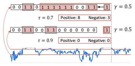
Note that this scheme is controlled by two design parameters: the actionness threshold and the tolerance threshold. The final proposal set is the union of those derived from individual combination of the two values. This scheme is called Temporal Actionness Grouping, illustrated in the above figure, which has several advantages:

1. Thanks to the actionness classifier, the generated proposals are mostly focused on action-related contents, which greatly reduce the number of needed proposals.
2. Action fragments are sensitive to temporal transitions. Hence, as a bottom-up method that relies on merging action fragments, it often yields proposals with more accurate temporal boundaries.
3. With the multi-threshold design, it can cover a broad range of actions without the need of case-specific parameter tuning. With these properties, the proposed method can achieve high recall with just a moderate number of proposals. This also benefits the training of the classifiers in the next stage.

Detecting Action Instances

this is accomplished by a cascaded pipeline with two steps: activity classification and completeness filtering.

Activity Classification

A classifier is trained based on TSN. During training, region proposals that overlap with a ground-truth instance with an IOU above 0.7 will be used as positive samples. A proposal is considered as a negative sample only when less than 5% of its time span overlaps with any annotated instances. Only the proposals classified as non-background classes will be retained for completeness filtering. The probability from the activity classifier is denoted as $P_{a}$.

Completeness Filtering

To evaluate the completeness, a simple feature representation is extracted and used to train class-specific SVMs. The feature comprises three parts: (1) A temporal pyramid of two levels. The first level pools the snippet scores within the proposed region. The second level split the segment into two parts and pool the snippet scores inside each part. (2) The average classification scores of two short periods – the ones before and after the proposed region. The method is illustrated in the following figure.

The output of the SVMs for one class is denoted as $S_{c}$.

Then final detection confidence for each proposal is

$$ S_{Det} = P_{a} \times S_{c} $$

Sunday was really sunny! Beautiful breakfast, beautiful day!

I said ten days ago that maybe I could make cakes in the futue. Then today I made this dream true. This is the first time that I made a cake, which seems to be not that hard and it brought me much sense of pleasure in this weekend.

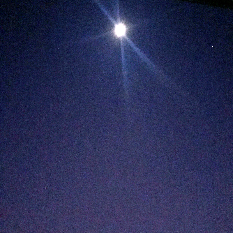
We can see the vague image of Orion right below the Moon and Alhena top left, Aldebaran top right, Sirius left bottom. I’ve not been looking at the stars for a long time! I can not even remember when was the last time I do that.

Orion was the first constellation that I learnt by reading a book telling stories and myths about the stars for kids. I was attracted by Orion because of the myth that how he became one of the constellations.

One myth recounts Gaia’s rage at Orion, who dared to say that he would kill every animal on the planet. The angry goddess tried to dispatch Orion with a scorpion. This is given as the reason that the constellations of Scorpius and Orion are never in the sky at the same time. However, Ophiuchus, the Serpent Bearer, revived Orion with an antidote. This is said to be the reason that the constellation of Ophiuchus stands midway between the Scorpion and the Hunter in the sky.

Another interesting thing is that the pyramids in Giza reflect the belt of Orion. I shared these stories with my classmates in senior school when I was giving a speech to the whole class. I think another reason that I like Orion is that I was born in winter and Orion has the brightest stars in winter.

TITLE: Understanding Convolution for Semantic Segmentation

AUTHOR: Panqu Wang, Pengfei Chen, Ye Yuan, Ding Liu, Zehua Huang, Xiaodi Hou, Garrison Cottrell

ASSOCIATION: UC San Diego, CMU, UIUC, TuSimpl

FROM: arXiv:1702.08502

CONTRIBUTIONS

1. A method called dense upsampling convolution (DUC) is proposed, which instead of trying to recover the full-resolution label map at once, an array of upscaling filters are learnt to upscale the downsized feature maps into the final dense feature map of the desired size.
2. A simple hybrid dilation convolution (HDC) framework is proposed, which instead of using the same rate of dilation for the same spatial resolution, a range of dilation rates are used and are concatenated serially the same way as “blocks” in ResNet-101.

METHOD

DUC is illustrated as the following figure.

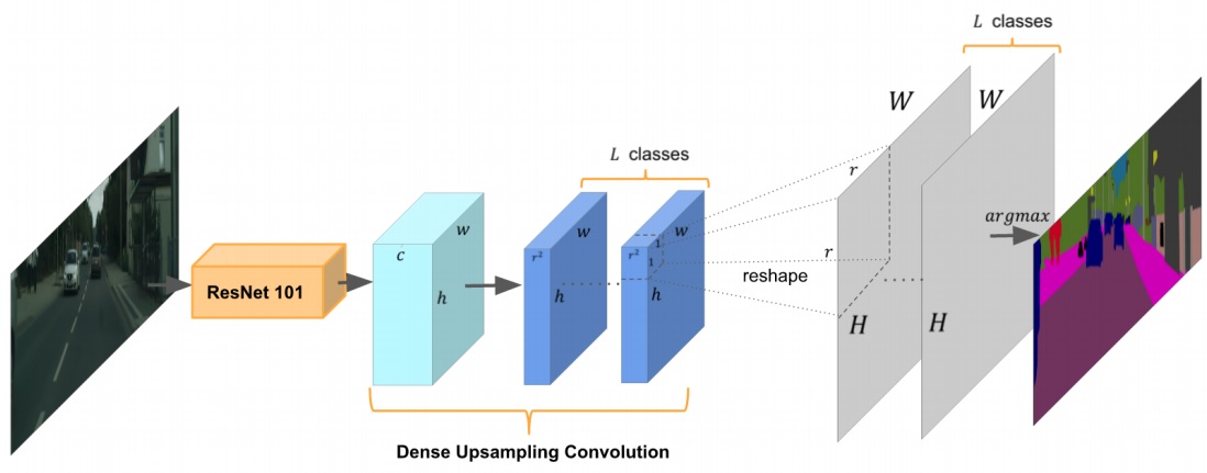
The key idea of DUC is to divide the whole label map into equal subparts which have the same height and width as the incoming feature map. Every feature map in the dark blue part is a corner or a part of the whole output.

HDC is illustrated as the following figure.

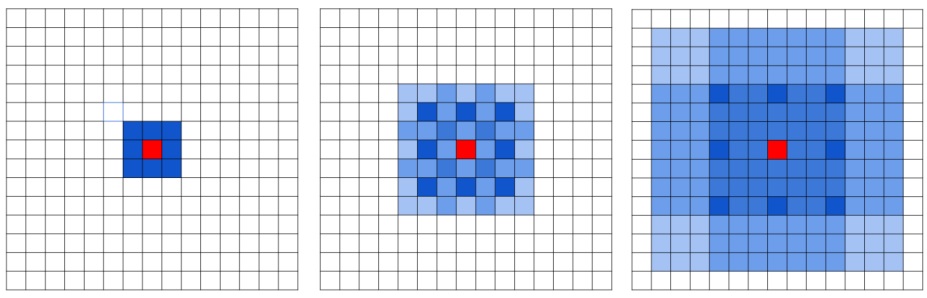
Instead of using the same dilation rate for all layers after the downsampling occurs, a different dilation rate for each layer is used. The pixels (marked in blue) contributes to the calculation of the center pixel (marked in red) through three convolution layers with kernel size 3 × 3. Subsequent convolutional layers have dilation rates of r = 1, 2, 3, respectively.

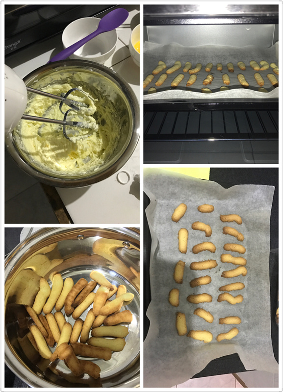
Wow~~~ It’s the first time that I baked something. Hmm… perhaps I should call them caterpillar cookies :) Maybe in the future I can make cakes.

TITLE: Learning to Detect Human-Object Interactions

AUTHOR: Yu-Wei Chao, Yunfan Liu, Xieyang Liu, Huayi Zeng, Jia Deng

ASSOCIATION: University of Michigan Ann Arbor, Washington University in St. Louis

FROM: arXiv:1702.05448

CONTRIBUTIONS

1. HICO-DET is introduced, a dataset that provides more than 150K annotated instances of human-object pairs covering the 600 HOI categories in HICO
2. A novel DNN-based framework for HOI detection is proposed. Human-Object Region-based Convolutional Neural Networks (HO-RCNN) outputs a pair of bounding boxes for each detected HOI instance. At the core of HO-RCNN is the Interaction Pattern, a novel DNN input that characterizes the spatial relations between two bounding boxes.

METHOD

HO-RCNN detects HOIs in two in two steps.

1. Proposals of human-object region pairs are proposed using human and object detectors.
2. Each human-object proposal is passed into a ConvNet to generate HOI classification scores.

The network adopts a multi-stream architecture to extract features on the detected humans, objects, and human-object spatial relations, as the following figure illustrated.

Human-Object Proposals

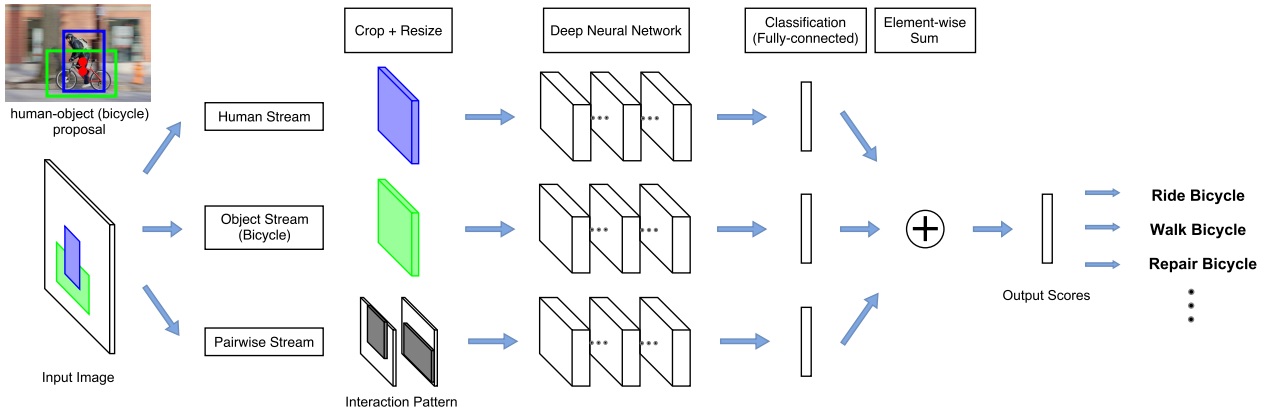
Assuming a list of HOI categories of interest (e.g. “riding a horse”, “eating an apple”) is given beforehand, bounding boxes for humans and the object categories of interest (e.g. “horse”, “apple”) are generated by detectors. Th human-object proposals are generated by pairing the detected humans and the detected objects of interest.

Multi-stream Architecture

The multistream architecture is composed of three streams

1. The human stream extracts local features from the detected humans.
2. The object stream extracts local features from the detected objects.
3. The pairwise stream extracts features which encode pairwise spatial relations between the detected human and object.

The last layer of each stream is a binary classifier that outputs a confidence score for the HOI. The final confidence score is obtained by summing the scores over all streams.

Human and Object Stream

An image patch is cropped according to the bounding box (human/object) and is resized to a fixed size. Then the image patch is sent to a CNN to be classified and given an confidence for a HOI.

Pairwise Stream

Given a pair of bounding boxes, its Interaction Pattern is a binary image with two channels: The first channel has value 1 at pixels enclosed by the first bounding box, and value 0 elsewhere; the second channel has value 1 at pixels enclosed by the second bounding box, and value 0 elsewhere. In this work, the first bounding box is for humans, and the second bounding box is for objects.

The Interaction Patterns should be invariant to any joint translations of the bounding box pair. The pixels outside the “attention window”, i.e. the tightest window enclosing the two bounding boxes, are removed from the Interaction Pattern. the aspect ratio of Interaction Patterns should be fixed. Two methods are used. One wrap the patch, the other one extend the shorter side of the patch to meet the required ratio.

To extend to mulitple HOI classes, one binary classifier is trained for each HOI class at the last layer of each stream. The final score is summed over all streams separately for each HOI class.

SOME IDEAS

1. Now the method is very similar with RCNN, maybe Fast-RCNN can also be used. Thus we can save much time for extracting features.
2. How to exclude the condition of known HOI categories?